Artificial
Intelligence 3E
foundations of computational agents


11.2 Missing Data
When data is missing some values for some features, the missing data cannot be ignored. Example 10.13 gives an example where ignoring missing data leads to wrong conclusions. Making inference from missing data is a causality problem, as it cannot be solved by observation, but requires a causal model.
A missingness graph, or m-graph for short, is used to model data where some values might be missing. Start with a belief network model of the domain. In the m-graph, all variables in the original graph exist with the same parents. For each variable that could be observed with some values missing, the m-graph contains two extra variables:
-
•
, a Boolean variable that is true when ’s value is missing. The parents of this node can be whatever variables the missingness is assumed to depend on.
-
•
A variable , with domain , where is a new value (not in the domain of ). The only parents of are and . The conditional probability table contains only 0 and 1, with the 1s being
If the value of is observed to be , then is conditioned on. If the value for is missing, is conditioned on. Note that is always observed and conditioned on, and is never conditioned on, in this augmented model. When modeling a domain, the parents of specify what the missingness depends on.
Example 11.5.
Example 10.13 gives a problematic case of a drug that just makes people sicker and so drop out, giving missing data. A graphical model for it is shown in Figure 11.5.
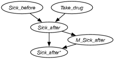
Assume is Boolean and the domains of and are , , . Then the domain of is , , , . The variable is Boolean.
Suppose there is a dataset from which to learn, with and observed for each example, and some examples have observed and some have it missing. To condition the -graph on an example, all of the variables except are conditioned on. has the value of when it is observed, and has value otherwise.
You might think that you can learn the missing data using expectation maximization (EM), with as a hidden variable. There are, however, many probability distributions that are consistent with the data. All of the missing cases could have value for , or they all could be ; you can’t tell from the data. EM can converge to any one of these distributions that are consistent with the data. Thus, although EM may converge, it does not converge to something that makes predictions that can be trusted.
To determine appropriate model parameters, one should find some data about the relationship between and . When doing a human study, the designers of the study need to try to find out why people dropped out of the study. These cases cannot just be ignored.
A distribution is recoverable or identifiable from missing data if the distribution can be accurately measured from the data, even with parts of the data missing. Whether a distribution is recoverable is a property of the underlying graph. A distribution that is not recoverable cannot be reconstructed from observational data, no matter how large the dataset. The distribution in Example 11.5 is not recoverable.
Data is missing completely at random (MCAR) if and are independent. If the data is missing completely at random, the examples with missing values can be ignored. This is a strong assumption that rarely occurs in practice, but is often implicitly assumed when missingness is ignored.
A weaker assumption is that a variable is missing at random (MAR), which occurs when is independent of given the observed variables . That is, when . This occurs when the reason the data is missing can be observed. The distribution over and the observed variables is recoverable by . Thus, the non-missing data is used to estimate and all of the data is used to estimate .
Example 11.6.
Suppose you have a dataset of education and income, where the income values are often missing, and have modeled that income depends on education. You want to learn the joint probability of and .
If income is missing completely at random, shown in Figure 11.6(a), the missing data can be ignored when learning the probabilities:
since is independent of and .
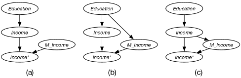
If income is missing at random, shown in Figure 11.6(b), the missing data cannot be ignored when learning the probabilities, however
Both of these can be estimated from the data. The first probability can ignore the examples with missing, and the second cannot.
If is missing not at random, as shown in Figure 11.6(c), which is similar to Figure 11.5, the probability cannot be learned from data, because there is no way to determine whether those who don’t report income are those with very high income or very low income. While algorithms like EM converge, what they learn is fiction, converging to one of the many possible hypotheses about how the data could be missing.
The main points to remember are:
-
•
You cannot learn from missing data without making modeling assumptions.
-
•
Some distributions are not recoverable from missing data, and some are. It depends on the independence structure of the underlying graph.
-
•
If the distribution is not recoverable, a learning algorithm still may be able to learn parameters, but the resulting distributions should not be trusted.
Artificial Intelligence: Foundations of Computational Agents, Poole
& Mackworth
Copyright © 2023, David L. Poole and Alan K. Mackworth. 
This work is licensed under a Creative Commons Attribution-NonCommercial-NoDerivatives 4.0 International License.